Modern Portfolio Theory in a nutshell
By Dimitrios Koulialias
I) Formulation of the Modern Portfolio Theory
The purpose of investing is to allocate an amount of money into one or more asset classes with the aim to get a higher reward back after a certain time. Investing your money with one click has nowadays never been that easy considering the myriad of web platforms through which you can place your order in a variety of assets, ranging from the classic stocks and bonds to more elaborate ones such as futures or derivatives. Before, however, placing your order, it is worth keeping in mind the golden rule to "not put all your eggs in one basket". Therefore, apart from money, it would be wise to also invest some time in order to estimate your investment strategy and the amount of risk you are willing to tolerate. In the following, I am going to provide you a simple procedure by which you can assess your optimal portfolio based on Modern Portfolio Theory (MPT).
The MPT has been put forward by the economist and nobel prize winner Harry Markowitz in 1952 and is still to date the most popular theory when it comes to investment decisions. It provides a general framework to construct an optimal portfolio for a given level of risk which is mathematically worked out as follows. Assume you want to invest your money in a number \(n\) of asset classes. Let us denote the allocation weights of the classes as \(w_i\) (\(0 \leq w_i \leq 1, i=1,2,...,n\)), with the condition that their sum constitutes 100 % of your invested capital, i.e., \(\sum_{i=1}^n w_i = 1\) (note that the \( w_i \) are non-negative, which means that we omit portfolios with shortselling). To determine your optimal allocation, there are three main quantities you need to encounter, which can be readily deduced from the gross daily returns \( \mu_{ik} \) of each of the assets: 1. The average return \( \overline{r_i} \), which indicates your asset's performance over \( N \) trading days \begin{equation*} \overline{r_{i}} = \frac{1}{N} \sum_{k=1}^N \mu_{ik} \end{equation*} 2. The risk or volatility \( \sigma_i \), which is a measure of the dispersion of returns with respect to \( \overline{r_i} \) and is generally represented by the standard deviation \begin{equation*} \sigma_i = \sqrt{\frac{\sum_{k=1}^N (\mu_{ik} - \overline{r_{i}})^2}{N-1}} \end{equation*} 3. The covariance \( \sigma_{ij} \), which is a measure of the correlated risk between asset \(i\) and \(j\). For the special case \(i=j\), it corresponds to the variance of the \(i\)-th stock, that relates to the standard deviation as \(\textnormal{Var}_i = \sigma_i^2 \). From these quantities, the portfolio's return \( r_{P} \) can be calculated, which is equal to the weighted sum of the average returns, i.e., \begin{equation} r_{P} = \sum_{i=1}^n w_i \overline{r_{i}}\tag{1} \end{equation} In contrast, the portfolio's risk \( \sigma_{P} \) is not equal to the average of the volatilities, but is given as \begin{equation} \sigma_{P} = \sqrt{\sum_{i=1}^n\sum_{j=1}^{n} w_i w_j \sigma_{ij}} \tag{2} \end{equation}
From eqns. (1) and (2), there are two ways you can construct your portfolio. If you are a risk-averse investor, then you would choose one allocation that minimizes \( \sigma_{P}\), but this would also yield the lowest expected return. On the other hand, if you are aiming for a higher expected return, you would be willing to take more risk, but you would need to find that allocation that results in an optimal balance between \( r_{P} \) and \( \sigma_{P}\). This allocation is retrieved via the Sharpe ratio (SR) defined as \begin{equation*} SR = \frac{r_P - r_f}{\sigma_P} \end{equation*} and can be considered as a measure of the excess risk you are undertaking with respect to a risk-free/low investment with rate \( r_{f} \). Due to the current restrictive interest policy imposed by several central banks, we can assume that the risk-free interest rate is essentially zero, which reduces the SR to \begin{equation} SR = \frac{r_P}{\sigma_P} \tag{3} \end{equation}
Considering the above, it becomes evident that the allocation either fulfilling \(\sigma_{P} \stackrel{!}{=}\) min. or \( \textnormal{SR} \stackrel{!}{=} \) max. along with the equality condition \(\sum_{i=1}^n w_i = 1\) is the solution of a constrained optimization problem. In the following, I am going to deduce the optimal allocations using a concrete example of asset classes.
II) Implementation of the MPT on a concrete example
While searching through the web, there are four assets that I'm interested in and in which I would like to invest. My portfolio should be a mix of exchange traded funds (ETF's), stocks, commodities, and cryptocurrencies. The individual components are shown in the following table:
| Asset Nr. | Asset Class | Product Name | Abbreviation |
|---|---|---|---|
| 1 | ETF | UBS - CMCI Oil SF (CH) A-dis | OILCHA.SW |
| 2 | Stocks | MongoDB | MDB |
| 3 | Commodities | Gold (per ounce) | GC=F |
| 4 | Cryptocurrencies | Bitcoin | BTC-USD |
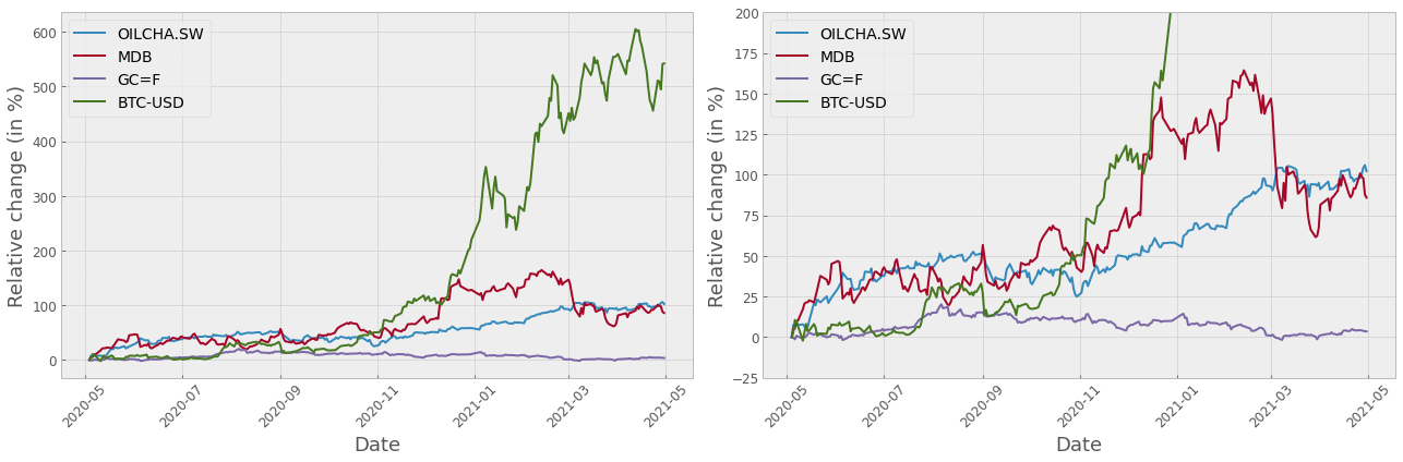
Fig. 1 shows an overview of their relative one-year performance between May 2020 and 2021. It is evident that Bitcoin is by far the riskiest asset, considering its exceptional performance it had during the last year. In the second run is MongoDB, followed by the UBS Oil ETF and Gold, which among the other assets shows a relatively stable behavior.
The first step for finding the optimal allocations relies on a Monte-Carlo simulation approach, which is associated with repeated random sampling. In our case, this means to repeteadly generate potrtfolios with random weights, of which we calculate their return, volatility, and the SR via eqns. (1) to (3). An implementation with 10'000 iterations yields the following return vs. risk diagram as depicted in Figure 2.
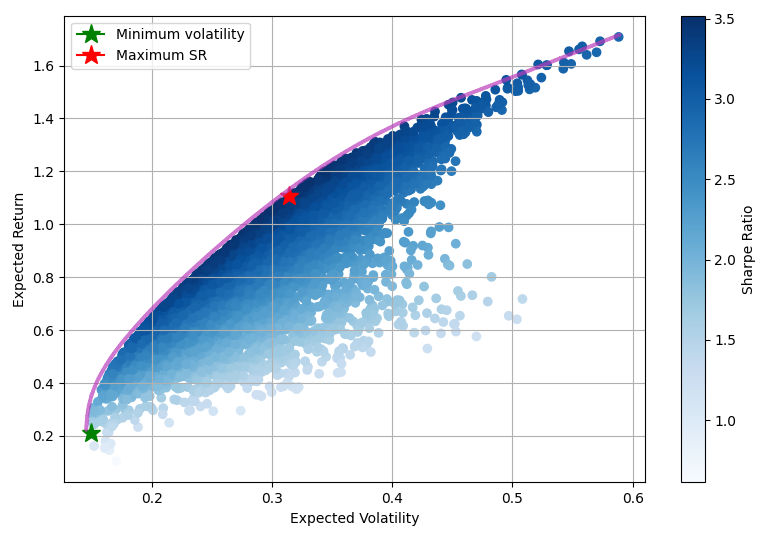
From the above plot, we now can calculate the optimal portfolios (the minimization processes can be readily implemented in Python. I am omitting here any details for simplicity). For the case \(\sigma_{P} \stackrel{!}{=}\) min., we get a return of 21.2 % and a volatility of 14.9 % along with the following allocation that corresponds to the outermost portfolio illustrated with a green star in Figure 2:
| Asset Nr. | Abbreviation | Allocation |
|---|---|---|
| 1 | OILCHA.SW | 22.6 % |
| 2 | MDB | 4.4 % |
| 3 | GC=F | 73.0 % |
| 4 | BTC-USD | 0 % |
From this portfolio, when we increase the level of risk, the highest expected return we can get is attained by those portfolios that constitute the upper boundary of the scatter plot, which is the so-called efficient frontier (Figure 2). Considering the case \(\textnormal{SR} \stackrel{!}{=}\) max., this portfolio is also an element of the efficient frontier and is equivalently retrieved by minimizing \( (-1) \cdot \textnormal{SR} \). The minimization yields SR = 3.52, with a return of 110.7 % and a volality of 31.4 %, that can be achieved with the following allocation:
| Asset Nr. | Abbreviation | Allocation |
|---|---|---|
| 1 | OILCHA.SW | 53.2 % |
| 2 | MDB | 11.7 % |
| 3 | GC=F | 0 % |
| 4 | BTC-USD | 35.1 % |
III) Discussion
The above analysis gave you an overview of the MPT in terms of the underlying mathematical concepts and its implementation based on a concrete choice of assets. The results show a strong difference between the risk-averse portfolio and the one with the maximum Sharpe ratio with respect to the allocations. Note that the former portfolio allocates more than two-third of your capital in gold, whereas the latter suggests an investment of a bit more than one-third to Bitcoin, which are very high positions. It is worth noting that these portfolios were obtained as general solutions out of the minimization process using \(\sum_{i=1}^n w_i = 1\) as the only constraint. They can, however, be further refined by imposing additional constraints on the individual allocations. For example, you may want to invest up to 10 % of your capital in gold, which is generally recommended as upper limit for precious metals and/or commodities. Or you may consider that Bitcoin is excessively risky, and therefore, you prefer to reduce your investment in a range between 5 and 15 % for that asset. By adding these additional constraints and combining the MPT with other classic approaches, such as fundamental and/or technical analysis, you have an invaluable tool that provides you with the best investment strategy. To conclude, please bear in mind that we have not considered any fees at all, which can have a significant impact on your return. Hence, the very last step you should do prior to investing, is to compare the range of possible fees (e.g., transaction costs, deposit costs, currency exchanges, etc.) that may significantly vary depending on your bank, investment platform, broker, etc. This will give you a clearer picture on the range of net returns that you can expect.
IV) SMI Portfolio tool
Finally, I would like to present you a portfolio selection tool that I implemented with Django and Python. With the above information, you can use it to construct your optimal portfolio (i.e., with the highest SR) by choosing a number of stocks among the Swiss Market Index (SMI). Check out the following link.