Finding the price range of the best-rated pizzas in Zurich: an example using MongoDB

By Dimitrios Koulialias

When it comes to pizza, there is a myriad of restaurants and pizzerias in Zurich you can go to. An overview of these can be found, e.g., at https://zuri.net, which is a local alternative to Google & co. Being one of the most expensive cities in the world, however, finding a relatively cheap pizza in Zurich is not that easy, given that some pizzas may even cost up to 35 CHF (approximately 38.50 USD)!! Hence, before ordering your favorite pizza, it might be worth having a closer look on the price range. In this blog, I am extracting the pizza price distribution from twenty-one restaurants, which have been listed as the best ones according to https://zuri.net/de/zurich/top-pizzerias.htm. I addressed this task using MongoDB, one of the most popular NoSQL databases, in combination with Python.

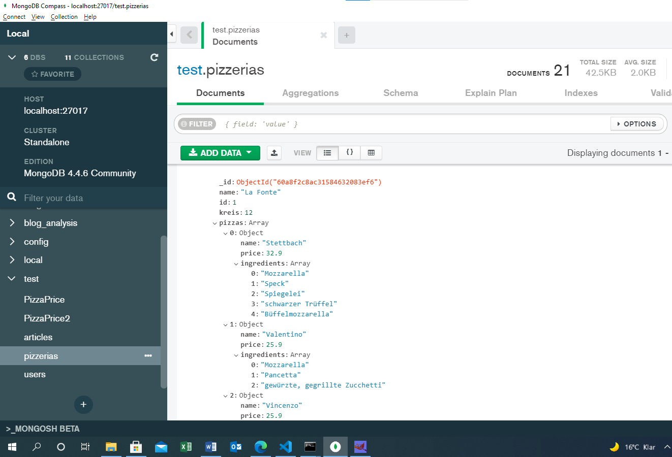
The database was created by importing the restaurant information, e.g., name and location, into MongoDB, along with the pizza names, prices, and ingredients that were inferred from the corresponding menus. Using MongoDB compass, a GUI for MongoDB, you can see that our database is called "test" and the restaurant/pizza information is stored in twenty-one documents within the collection termed as "pizzerias" (Fig. 1). Each restaurant is assigned to one document that contains a unique ObjectID automatically generated by MongoDB. The document further contains a restaurant id (for simplicity represented by a more readable, unique integer number next to the ObjectID), its name, and its location in terms of the city district number. The pizzas in turn are stored in an array as subdocuments, which contain the names, prices, and their ingredients, with the latter being stored in another array.

Fig. 1) Selected overview of the "test" database with the "pizzerias" collection in MongoDB compass.

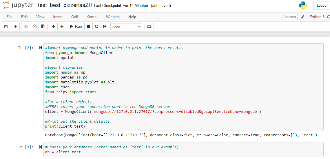
To search through the database, you can either make queries in MongoDB via the command shell, or directly through MongoDB Compass. Here, I prefer using Jupyter Notebook to combine MongoDB along with Python, which is quite suitable for directly visualizing the results from our queries. In the first notebook cell, I am importing pymongo and instantiate a client object to the connection port of the MongoDB shell via MongoClient (Fig. 2). I then assign a variable called "db" to the "test" database. To list all documents of the "pizzerias" collection, the general command in MongoDB is simply "db.pizzerias.find({})", which is equivalent to the SQL command "SELECT * FROM pizzerias". In contrast to the MongoDB shell, where the result is printed out right after this command, we need to additionally convert the result into a list and include pprint for printout in Jupyter Notebook. The third cell in Figure 2 shows the result, and you can see that that the printout starts with the entries of the first document, which corresponds to the restaurant "La Fonte" in accordance to Figure 1.

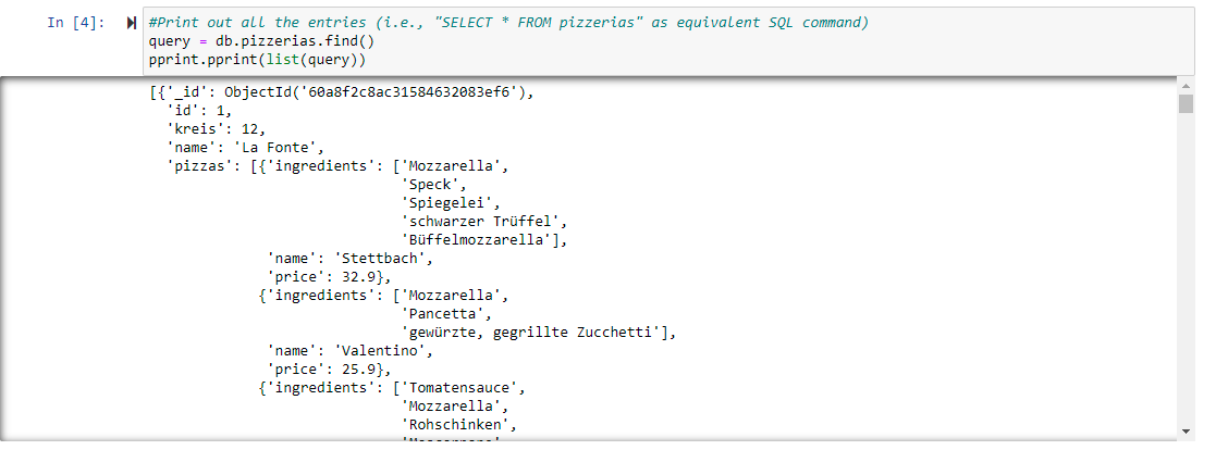
Fig. 2) Jupyter notebook with cells nr. 1-3

From all pizzas in the database, to plot the price range as a histogram, we need to make a query to extract the prices and their number of counts. The "find" command, corresponding to one of the main CRUD (create, read, update, delete) operations, is quite sufficient for retrieving documents if your database has a relatively simple structure. In our case, however, the individual prices of the pizzas are stored as subdocuments within an array, and therefore, we need to undertake a more elaborate approach to extract them. Specifically, we generate a series of stages, i.e., a pipeline, where the result of each stage is forwarded as input to the subsequent one, until we reach the desired output from the last stage (Fig. 3).

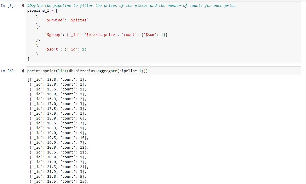
Fig. 3) Schematic illustration of the pipeline concept

This process is generally accomplished using the "aggregate" command as "db.pizzerias.aggregate(pipeline)", where "pipeline" is an array that contains the series of queries to be executed in particular order. In Figure 4, the "pipeline_I" array defined in the fourth cell provides us with the expected result, and the individual queries are explained as follows:

i) We split the main document into a series of subdocuments by pulling out the entries of the "pizzas" array. This is accomplished using the '$unwind' command.

ii) Next, we go through these subdocuments using the '$group' command, which contains the two fields of variables to be stored. By default, '$group' requires one variable to be specified as '_id', which in our case corresponds to the pizza price that is now easily retrieved via '$pizzas.price'. The second variable is the number of counts, which is built using the command 'count' : {'$sum': 1}.

iii) Finally, using '$sort': {'_id': 1}, we sort the result by the prices in ascending order.

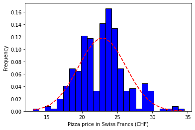
Fig. 4) Execution of pipeline_I and the printout of the prices (in CHF) with the number of counts

The histogram of this result is displayed in Figure 5 and can be best described with a normal distribution having a mean price $ \mu = 22.90 $ CHF and a standard deviation $ \sigma = 3.40 $ CHF.

Fig. 5) Pizza price histogram. The red dashed line indicates a standard normal distribution with $ \mu = 22.90 $ CHF and $ \sigma = 3.40 $ CHF.

Given the above, let us write a final pipeline to extract your favorite pizzas and see whether they are good value for money. For example, let’s assume that you like pizza with Gorgonzola cheese on top (which is my absolute favorite too!!). You can retrieve these pizzas using “pipeline_II” of Figure 6, with the individual queries being set as follows:

i) Similar to "pipeline_I", we again use '$unwind' to split the main document into a series of subdocuments.

ii) Among the subdocuments, we select those where 'Gorgonzola' is an element of the ingredients (note that I’m querying through the ingredients rather than the pizza name, considering that some pizzas that contain Gorgonzola are not necessarily named as such and/or may contain additional ingredients). This is accomplished by applying '$match' to 'pizzas.ingredients': 'Gorgonzola'. Moreover, we also want to extract those pizzas that cost less than or equal to the mean price $ \mu $, which are retrieved by the second command 'pizzas.price': {'$lte': mean}.

iii) Finally, we only want to display the restaurant’s name, as well as the name of the pizza along with the price. This is achieved using the '$project' command.

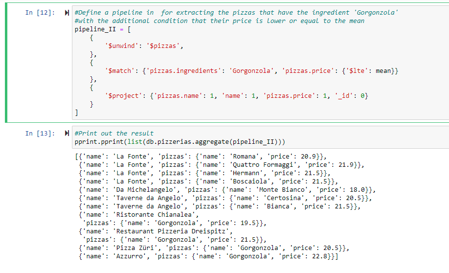
Fig. 6) Final results from "pipleine_II"

Finally, you can see that there are eleven pizzas with Gorgonzola that cost below the mean price of 22.90 CHF. If we further constrain our query to look for pizzas below the lower limit $ \mu - \sigma = $ 19.50 CHF, then there is the 'Monte Bianco' one left with 18.00 CHF. Buon appetito!